Case Description
Our client’s request was to implement a dynamic RLS. We had proper table specifying username and authorization pairings/access rights. Based on the business needs a hierarchical management had to be implemented, something like this:
- Country
- City
- Employee
In the fact tables each row includes a worker ID and a city ID. It is geographically assured that a certain city belongs to a certain country within the defined period. Based on the client’s request the rules for the visibility of fact and dimensional data are:
- Senior managers can see the data of one or more country’s data (and their cities) and the data of the workers who work there
- Area managers and sales manegers can see the data of one or more cities and the workers who work there
- Employees can see their own data
- There are administrators who can see everything
- There may be employees who, apart from seeing their own data, can also see data generated in a city (eg sales and area manager at the same time).
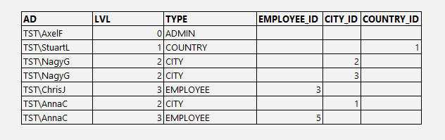
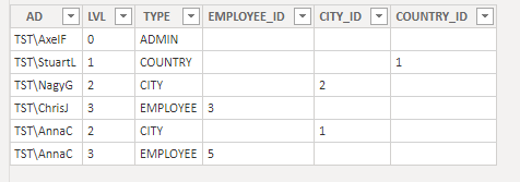
This is the summary what we see in the logic that serves the RLS:
The problem
- The occasionally necessary many-to-many connections are easily doable using intermediate tables, but this approach is far from ideal in terms of modeling and performance.
- A special problem are the users who “appear” in two categories/on two levels (the last two rows in the table above), because in their case you need to filter two dimensional tables, but due to the AND relationship of the filters, the user permission are not extended, but narrowed down, so instead of having a combination of the two data sets you only get a section of it.
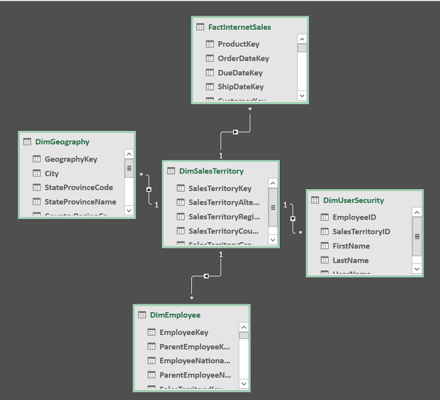
The extended model (seen below) shows that an additional problem is the visibility of related dimension data, for example, the cities or countries dimension does not filter employee data, i.e. it is not guaranteed that a manager with city-level authority will only see the master data for employees who worked in his city
It is guaranteed that you will be lost among the various many-to-many switchboards and even if you do it, still:
• It is complicated
• therefore, it is difficult to test
• any corrections or modification carry a huge risk
The solution
Principles
Leaving behind our habits and past modeling practices, we have laid down new principles that provide a solution to the business need without over-complicating the model or the whole process:
- We used a single dimension table to filter based on fact RLS conditions: Country, City, Employee
- We used a single table containing user data to define the RLS: UserId, Access level etc.
- Given that the number of returned value sets is low (filter for less than 10 country / city / employee IDs), we allowed ourselves to use DAX filters instead of m2m relationships in the model.
Preparation
Fact and dimension
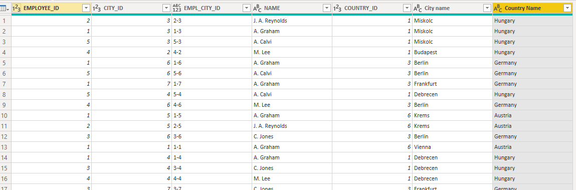
You need to generate an unique identifier in the fact and dimension tables that ensures the transfer of RLS filters, which ensure that a city can belong to a country, so that the employee ID and the city will be connected:
concat([employee_id],’-’,[City_ID])
The source of the dimension table can be the fact table queried using distinct, or in the case of a corresponding HR strain, an extract of it. It is important that an identifier appears only once in the new dimension table and that the table must contain the data to be used in the report, eg name, telephone number, city coordinates, etc.
In case of more detailed demand it can be supplemented with validity management, and a period identifier can be appended to the identifier.
Viewed in PowerQuery, our dimension table will look like this:
The RLS table will be the summary table shown at the beginning:
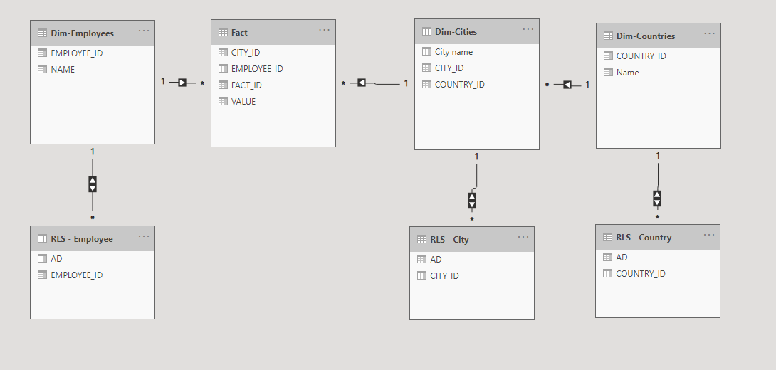
Based on this the new model will be much more simple and clear
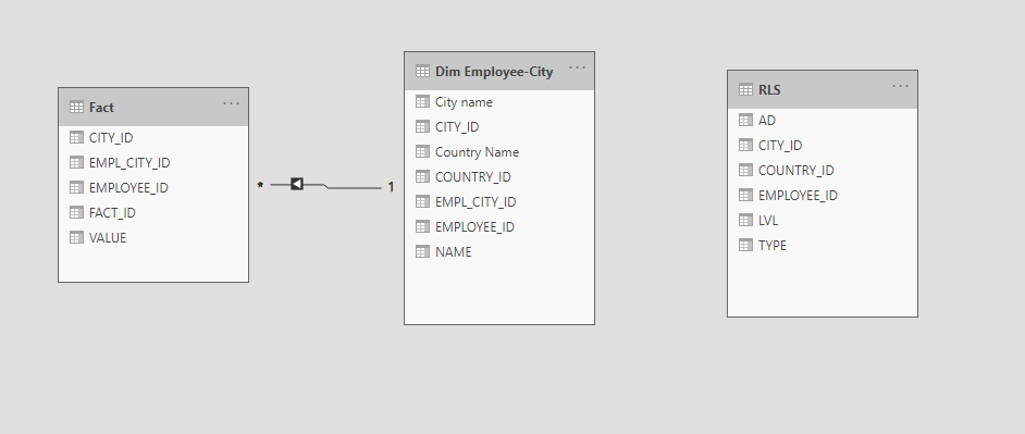
The new model contains:
- all RLS data
- all employee data
- every city
- data for all countries
- the factual data to be examined, with a simple relationship
DAX Role Filtering
Basis
We assume that the access levels have separate AD groups, so the Role containing 3 filters can be added separately (at the end we will examine what if they don’t).
Logic
Filtering for Country:
The dimension table must be filtered for the rows that contain the country IDs that appear next to the user ID in the RLS table:
Conversely:
Collecting the country ID-s related to the users from the RLS
var usercountries=calculatetable(values(’RLS’[COUNTRY_ID]), ’RLS’[AD]=username()))
Dimension filtering for these ID-s:
filter(’Dim Employee-City’, ’Dim Employee-City’[COUNTRY_ID] in usercountries)
Implementation
Rules added to the Dim Employee-City table.
Country:
’Dim Employee-City’[COUNTRY_ID] in calculatetable(values(’RLS’[COUNTRY_ID]), ’RLS’[AD]=username()))
City:
’Dim Employee-City’[CITY_ID] in calculatetable(values(’RLS’[CITY_ID]), ’RLS’[AD]=username()))
Employee:
’Dim Employee-City’[EMPLOYEE_ID] in calculatetable(values(’RLS’[EMPLOYEE_ID]), ’RLS’[AD]=username()))
If there are no separate AD groups
The three rules can be combined into one.
’Dim Employee-City’[COUNTRY_ID]
in calculatetable(values(’RLS’[COUNTRY_ID]), ’RLS’[AD]=username()))
||
’Dim Employee-City’[CITY_ID]
in calculatetable(values(’RLS’[CITY_ID]), ’RLS’[AD]=username()))
||
’Dim Employee-City’[EMPLOYEE_ID]
in calculatetable(values(’RLS’[EMPLOYEE_ID]), ’RLS’[AD]=username()))
Summary (Lessons learned)
Although it is basic rule that we solve problems in a model or data source preferring SQL, aiming for the simplicity in case of DAX formulas, here from the model’s usability point of view the complex solution is less resource intensive:
- working with two tables instead of using a complex model
- we ensure low result numbers during RLS filtering (eg it does not return the ID of all employees in the country, but only 1-2 country codes or 1-2 cities)
- the model remains simple, stable
- We were able to create a general solution for the customer and subsequently this RLS solution has become a standard for several other data sets with similar / identical dimensional resolution.
The lesson of the solution is that many complex problems can be solved within the Microsoft BI ecosystem, no matter what tool we are using (SQL, .NET, Tabular or DAX), we just don’t need be afraid to step out of our schemas, standards, and try to think “outside the box” to find the ideal solutions.